Gaussian Mixture Models

In unsupervised learning, Gaussian Mixture Models (GMM) are strong statistical models that simulate data generated from a combination of multiple Gaussian distributions, each representing a potential cluster. GMM may describe more sophisticated clustering patterns than techniques like K-Means since the data points are assigned to various Gaussian components according to probability. In GMM, each cluster has a weight representing its percentage in the whole mixture, along with a mean and variance. GMM’s probabilistic methodology makes it adaptable to real-world scenarios by modeling various sizes and forms of clusters.

Key Concepts of Gaussian Mixture Models:

Gaussian Distribution (Normal Distribution)

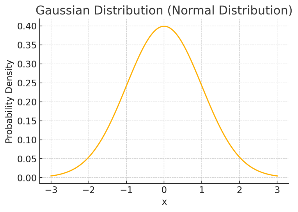
$$ f(x|\mu, \sigma^2) = \frac{1}{\sqrt{2\pi\sigma^2}} \exp\left(-\frac{(x – \mu)^2}{2\sigma^2}\right) $$ The formula above represents the probability density function (PDF) of the normal distribution. In this context, $ \mu $ is the mean of the distribution, acting as the center of the bell curve. The parameter $ \sigma^2 $ denotes the variance, which indicates the spread or width of the curve; larger values of $ \sigma^2 $ result in a broader, flatter distribution, while smaller values create a narrower curve. The exponential function, $ \exp $, is crucial in determining how quickly the probability decreases as $ x $ deviates from the mean. The mathematical constant $ \pi $ (approximately 3.14159) is part of the normalization factor to ensure the total area under the curve equals one. This formula defines the classic bell shape of the normal distribution, where the peak occurs at $ x = \mu $, and the curve symmetrically decreases as $ x $ moves further from $ \mu $. The normal distribution diagram is presented in Figure 1.

Figure 1

Practical example:

Take the example of a school where we wish to model the height distribution of children to determine whether it follows a Normal Distribution. Through the analysis of this data, we can answer questions like:

What is the average height of the students?
How much do students’ heights vary (standard deviation)?
What percentage of students are taller or shorter than a given height?

Step-by-step:

Randomly generate data for students’ heights.
Calculate the mean and standard deviation of the data.
Visualize the distribution of heights.
Calculate probabilities for specific height ranges.

import numpy as np
import matplotlib.pyplot as plt
from scipy.stats import norm

# Step 1: Generate synthetic height data (in cm)
np.random.seed(42)
mean_height = 170  # mean height in cm
std_dev_height = 10  # standard deviation in cm
height_data = np.random.normal(mean_height, std_dev_height, 1000)

# Step 2: Fit a Gaussian distribution to the data to find the mean and standard deviation
mu, std = norm.fit(height_data)

# Step 3: Plot the histogram of the data and the fitted distribution
plt.figure(figsize=(10, 6))
plt.hist(height_data, bins=30, density=True, alpha=0.6, color='skyblue', label='Height Data Histogram')

# Plot the fitted normal distribution
xmin, xmax = plt.xlim()
x = np.linspace(xmin, xmax, 100)
p = norm.pdf(x, mu, std)
plt.plot(x, p, 'r', linewidth=2, label=f'Fitted Normal Distribution\n(mean={mu:.2f}, std={std:.2f})')

# Labels and legend
plt.title('Height Distribution of Students')
plt.xlabel('Height (cm)')
plt.ylabel('Density')
plt.legend()
plt.show()

# Step 4: Calculate probabilities
# Probability of being taller than 180 cm
prob_taller_180 = 1 - norm.cdf(180, mu, std)
print(f"Percentage of students taller than 180 cm: {prob_taller_180 * 100:.2f}%")

# Probability of being shorter than 160 cm
prob_shorter_160 = norm.cdf(160, mu, std)
print(f"Percentage of students shorter than 160 cm: {prob_shorter_160 * 100:.2f}%")

Explanation:

Generate synthetic height data: We use np.random.normal() to create 1000 data points simulating students’ heights, assuming a normal distribution with a mean of 170 cm and a standard deviation of 10 cm.
Fit the data: We use norm.fit() to estimate the mean and standard deviation from the data.
Visualize the distribution: We create a histogram of the heights and overlay a red line showing the fitted normal distribution curve.
Calculate probabilities:
- We use norm.cdf() to find the cumulative probability of being shorter than a specific height (e.g., 160 cm).
- We subtract the cumulative probability from 1 to find the probability of being taller than a specific height (e.g., 180 cm).

Mixture Model

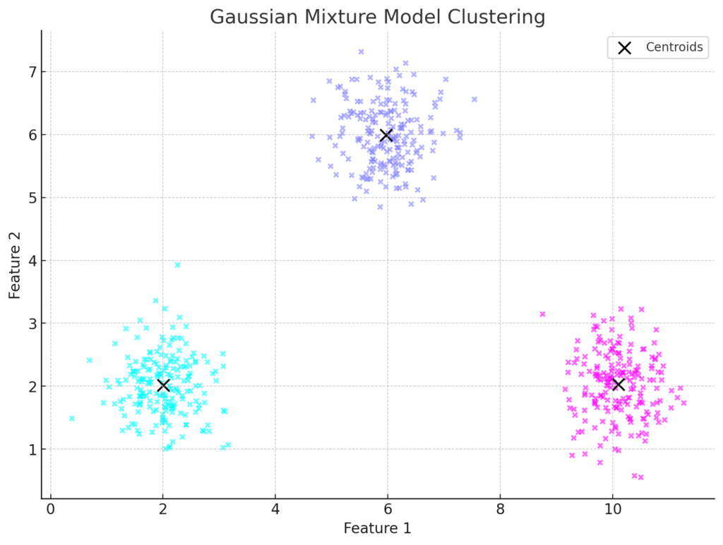
This model is used for clustering by assuming that data points are generated from a mixture of several Gaussian distributions. The probability density function for GMM is given by:$$p(x) = \sum_{i=1}^{K} \phi_i \mathcal{N}(x | \mu_i, \sigma_i)$$ where $K$ is the number of Gaussian components (clusters), $\phi_i$ represents the weight of the $i$th Gaussian component (such that $\sum_{i=1}^{K} \phi_i = 1$), $\mathcal{N}(x | \mu_i, \sigma_i)$ is the Gaussian distribution with mean $\mu_i$ and covariance $\sigma_i$. The plot above illustrates the GMM clustering results, showing data points assigned to different Gaussian components, with centroids marked as black crosses, as shown in Figure 2. This model effectively models clusters with various shapes, sizes, and orientations.

Figure 2

Practical example:

In this example, we will find customer segmentation in marketing as a real-world example of a Mixture Model. Imagine an e-commerce company that wants to segment its customers based on their annual spending and number of purchases. The company believes customers may belong to different groups (e.g., low, medium, and high spenders), each with its own characteristics. Using a GMM, we can identify these segments and model the data as a mixture of Gaussian distributions.

What to find:

Customer Segments: Group customers into clusters based on their spending and purchase frequency.
Means and Covariances of Clusters: Identify the average characteristics of each customer segment.
Cluster Weights: Determine the proportion of customers in each segment.

Step-by-step:

Generate or load sample data for customer spending and purchases.
Fit a GMM to the data.
Visualize the clustered data.
Analyze the characteristics of the clusters.

import numpy as np
import matplotlib.pyplot as plt
from sklearn.mixture import GaussianMixture

# Step 1: Generate synthetic data for customer spending and number of purchases
np.random.seed(42)
cluster_1 = np.random.multivariate_normal([50, 5], [[30, 5], [5, 2]], 200)  # Low spenders
cluster_2 = np.random.multivariate_normal([150, 15], [[40, 5], [5, 5]], 200)  # Medium spenders
cluster_3 = np.random.multivariate_normal([300, 25], [[50, 10], [10, 3]], 200)  # High spenders
data = np.vstack((cluster_1, cluster_2, cluster_3))

# Step 2: Fit a Gaussian Mixture Model (GMM) to the data
gmm = GaussianMixture(n_components=3, random_state=42)
gmm.fit(data)
labels = gmm.predict(data)

# Step 3: Visualize the clustered data
plt.figure(figsize=(12, 8))
plt.scatter(data[:, 0], data[:, 1], c=labels, cmap='viridis', s=50, alpha=0.6, label='Data Points')
plt.scatter(gmm.means_[:, 0], gmm.means_[:, 1], c='red', marker='x', s=200, label='Cluster Centers')

plt.title('Customer Segmentation using Gaussian Mixture Model')
plt.xlabel('Annual Spending ($)')
plt.ylabel('Number of Purchases')
plt.legend()
plt.show()

# Step 4: Print cluster means and weights
print("Cluster Means (Annual Spending, Number of Purchases):")
print(gmm.means_)
print("\nCluster Weights (Proportion of Customers in Each Segment):")
print(gmm.weights_)

Explanation:

Generate synthetic customer data:
- We use np.random.multivariate_normal() to create data for three customer segments (low, medium, and high spenders) with different means and covariance matrices.
Fit the GMM to the data:
- We use GaussianMixture() from sklearn.mixture to fit the data and find the optimal parameters for the mixture model.
- The predict() method assigns each data point to the most probable cluster.
Visualize the clustered data:
- We use plt.scatter() to plot and color the data points based on their cluster assignment.
- Cluster centers are marked with red crosses.
Print cluster characteristics:
- The means_ attribute of the GMM provides each cluster’s mean values (centroids).
- The weights_ attribute provides the proportion of customers in each segment, indicating the relative size of each cluster.

Expectation-Maximization (EM) Algorithm

The algorithm alternates between two main steps:

Expectation Step (E-Step): In this step, the algorithm estimates the expected value of the latent variables given the current parameters of the model and the observed data. It calculates the probability that each data point belongs to each model component.
Maximization Step (M-Step): In this step, the algorithm updates the model parameters (e.g., means, variances, and mixture weights) to maximize the likelihood of the observed data based on the probabilities calculated in the E-step.

The formula for the EM Algorithm
- For a Gaussian Mixture Model (GMM), the EM algorithm updates the parameters iteratively as follows:
  - In the E-step, the responsibility $ \gamma_{i,k}$ for data point $x_i$ with respect to component $k$ is calculated as: $$ \gamma_{i,k} = \frac{\phi_k \mathcal{N}(x_i | \mu_k, \sigma_k)}{\sum_{j=1}^{K} \phi_j \mathcal{N}(x_i | \mu_j, \sigma_j)} $$
  - M-Step: Update the parameters $\mu_k$, $\sigma_k$, and $\phi_k$ using the responsibilities:
    - Update the mean $\mu_k$:$$\mu_k = \frac{\sum_{i=1}^{N} \gamma_{i,k} x_i}{\sum_{i=1}^{N}\gamma_{i,k}}$$
    - Update the covariance $\sigma_k^2$:$$\sigma_k^2 = \frac{\sum_{i=1}^{N}\gamma_{i,k} (x_i – \mu_k)^2}{\sum_{i=1}^{N}\gamma_{i,k}}$$
    - Update the weight $\phi_k$:$$\phi_k = \frac{\sum_{i=1}^{N} \gamma_{i,k}}{N}$$
Explanation of the Steps:
- E-Step: The algorithm calculates the probability (responsibility) that each data point belongs to each Gaussian component. This responsibility tells us how likely it is that a particular mixture component generated a data point.
- M-Step: The algorithm updates the model’s parameters (means, variances, and mixture weights) based on the responsibilities calculated in the E-step to better fit the observed data.
Diagram of EM Algorithm Process
- Initial positions of Gaussian components.
- E-step: Visualization of responsibilities where each data point is assigned to an element probabilistically.
- M-step: Adjustment of the means, variances, and weights to maximize the likelihood.

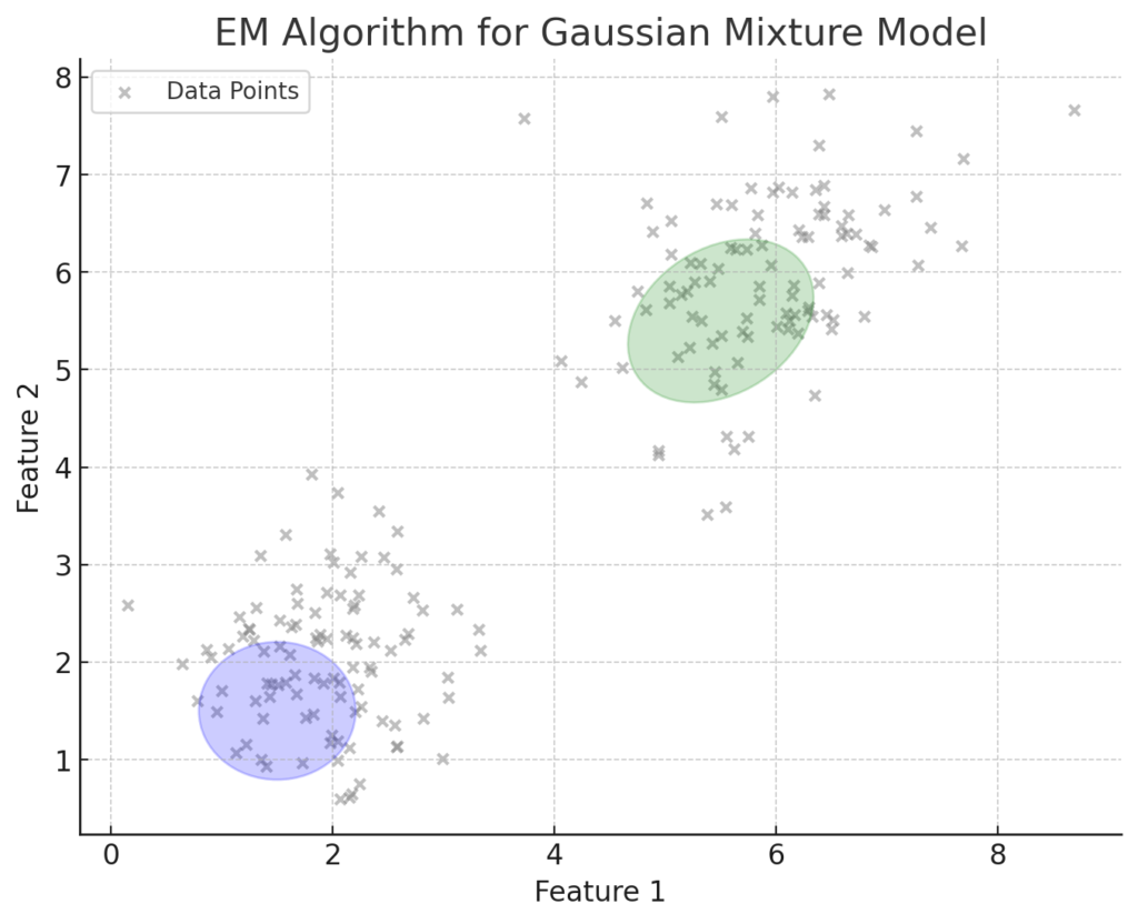
Figure 3 illustrates the initial step of the Expectation-Maximization (EM) algorithm for a Gaussian Mixture Model (GMM). It shows the initial positions of two Gaussian components overlaid on the data points. In the E-step, responsibilities for each data point relative to each element are computed. In the M-step, the means and covariances of these components will be updated based on these responsibilities. This iterative process continues until the parameters converge, optimizing the model’s fit to the data.

Figure 3

Practical example:

A practical example of using the Expectation-Maximization (EM) Algorithm is in image segmentation. For instance, in medical imaging, EM can separate different tissues based on their pixel intensities in an MRI scan. The algorithm can group pixels into different segments, representing tissues (e.g., bone, muscle, and fat).

What to find:

Segmentation of Image Pixels: Identify different pixel groups based on intensity values.
Mean and Variance of Each Segment: Understand each segment’s average intensity and variability.
Probability Assignments: Calculate the probability that a pixel belongs to each segment.

Step-by-step:

Load sample image data and convert it into pixel intensity values.
Use the EM algorithm through a Gaussian Mixture Model (GMM) to fit the data.
Assign pixels to the most probable segments.
Visualize the segmented image.

import numpy as np
import matplotlib.pyplot as plt
from sklearn.mixture import GaussianMixture
from skimage import data, color

# Step 1: Load a sample image and convert it to grayscale
image = color.rgb2gray(data.astronaut())  # Load an example image
pixels = image.flatten().reshape(-1, 1)  # Convert image to 1D array of pixel intensities

# Step 2: Fit a Gaussian Mixture Model (GMM) using the EM algorithm
gmm = GaussianMixture(n_components=3, random_state=42)  # Assume 3 components (e.g., tissue types)
gmm.fit(pixels)
labels = gmm.predict(pixels)

# Step 3: Reshape the labels to the original image shape for visualization
segmented_image = labels.reshape(image.shape)

# Step 4: Visualize the original and segmented images
fig, ax = plt.subplots(1, 2, figsize=(14, 7))
ax[0].imshow(image, cmap='gray')
ax[0].set_title('Original Image')
ax[0].axis('off')

ax[1].imshow(segmented_image, cmap='viridis')
ax[1].set_title('Segmented Image using EM Algorithm')
ax[1].axis('off')

plt.show()

Explanation:

Load sample image data:
- We use the astronaut image from skimage.data as a sample and convert it to grayscale using color.rgb2gray() to simplify the pixel intensity data.
- The pixel intensities are flattened into a 1D array to fit with the GMM.
Fit the GMM using the EM algorithm:
- The GaussianMixture() class from sklearn.mixture is used to create and fit the GMM, which runs the EM algorithm to find the optimal means, variances, and weights for the pixel intensities.
Segment the image:
- The predict() method assigns each pixel to a component based on its intensity and the GMM model.
- The segmented image is reshaped to match the original image’s dimensions.
Visualize the results:
- We use matplotlib.pyplot to display the original and segmented images side by side.