One type of unsupervised learning used for clustering and data visualization is Self-Organizing Maps (SOM). SOMs preserve the topological structure of high-dimensional data by mapping it to a lower-dimensional grid, usually 2D. They are useful for tasks like pattern identification, anomaly detection, and grouping because they make complex correlations in data easier to see.
Key concepts:
- Competitive Learning: Unlike traditional neural networks, SOMs use competitive learning, where neurons compete to represent input data.
- Neighborhood Function: Ensures that the neurons close to the winning neuron in the grid are updated during training, maintaining the topological structure.
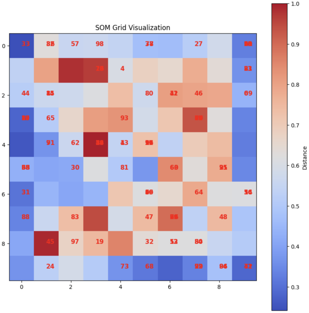
The SOM grid visualization diagram is shown in Figure 1.

Figure 1
Formulas:
- Distance Calculation: $d(i, x) = | w_i – x |$ , where ( w_i ) is the weight vector of neuron ( i ), and ( x ) is the input vector.
- Weight Update Rule: $w_i(t + 1) = w_i(t) + \eta(t) \cdot h_{ci}(t) \cdot (x(t) – w_i(t))$
- $\eta(t)$ : learning rate
- $h_{ci}(t)$ : neighborhood function centered around the winning neuron ( c )
Practical example:
Consider a dataset of customer purchase behavior in an e-commerce store. SOM can map customers with similar purchasing patterns to neighboring nodes, helping identify customer segments for targeted marketing campaigns.
Step-by-step:
- Load and preprocess the data
- Initialize the SOM and train it
- Visualize the results
!pip install minisom
import numpy as np
import matplotlib.pyplot as plt

#The MiniSom library is a Python tool for implementing Self-Organizing Maps (SOMs) to visualize, cluster, and analyze high-dimensional data unsupervised.
from minisom import MiniSom

# Step 1: Generate synthetic data (e.g., customer purchasing data)
np.random.seed(42)
data = np.random.rand(100, 2)  # 100 data points with 2 features each

# Step 2: Initialize the SOM
som = MiniSom(x=10, y=10, input_len=2, sigma=1.0, learning_rate=0.5)
som.random_weights_init(data)

# Step 3: Train the SOM
som.train_random(data, num_iteration=100)

# Step 4: Visualize the SOM grid
plt.figure(figsize=(10, 10))
for i, x in enumerate(data):
    winner = som.winner(x)
    plt.text(winner[0], winner[1], str(i), color='red', fontdict={'weight': 'bold', 'size': 11})
plt.imshow(som.distance_map().T, cmap='coolwarm', interpolation='nearest')
plt.colorbar(label='Distance')
plt.title('SOM Grid Visualization')
plt.show()
Explanation:
- Generate data: We create a synthetic dataset of 100 points with two features each.
- Initialize SOM: We create a 10×10 grid SOM using MiniSom with an input length of 2 (matching the data features).
- Train SOM: We train the SOM with num_iteration=100, where the SOM adjusts its weights to map the input data onto the grid.
- Visualize results: The trained SOM is visualized, with each data point mapped to its closest neuron. The grid’s color indicates the distance between neighboring neurons, with darker colors representing larger distances.

