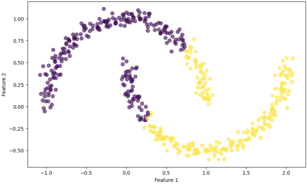
Spectral Clustering is an unsupervised learning algorithm used for clustering data points that are not linearly separable. It leverages the eigenvalues (spectrum) of the similarity matrix of the data to reduce dimensionality before clustering. Spectral clustering is particularly useful for data with complex cluster shapes, where traditional algorithms like K-Means may fail. A spectral clustering graph is shown in Figure 1.
Key Concepts:
- Similarity Matrix: A matrix representing the similarity between data points. Commonly constructed using Gaussian (RBF) kernel or k-nearest neighbors.
- Graph Representation: Every data point is a node in the graph, and edges connect nodes according to how related they are.
- Laplacian Matrix: This matrix is utilized for spectrum analysis and is built from the similarity matrix.
- Eigenvectors: The eigenvectors of the Laplacian matrix are used to reduce the dimensionality of the data for clustering.

Figure 1
Formulas
- Construct the Similarity Matrix $S$: $S_{ij} = \exp\left(-\frac{|x_i – x_j|^2}{2\sigma^2}\right)$ , where $ |x_i – x_j| $ is the Euclidean distance between points $ i $ and $ j $, and $ \sigma $ is a scaling parameter.
- Construct the Laplacian Matrix $L$: $L = D – S$, where $ D $ is the degree matrix (diagonal matrix with $D_{ii} = \sum_j S_{ij}$ ).
- Eigenvalue Decomposition: : Find the first $ k $ eigenvectors of $ L $ (corresponding to the $ k $ smallest eigenvalues) to form a new feature space.
- Apply Clustering: Run a standard clustering algorithm (e.g., K-Means) on the new feature space.
Practical Example:
Imagine segmenting images based on color similarity. Spectral clustering can group pixels into regions of similar colors, which is useful for image segmentation.
Step-by-step:
- Load a dataset
- Construct the similarity matrix
- Compute the Laplacian matrix and perform eigenvalue decomposition
- Cluster the data using K-Means on the reduced feature space
- Visualize the results
import numpy as np
import matplotlib.pyplot as plt
from sklearn.cluster import SpectralClustering
from sklearn.datasets import make_moons

# Step 1: Generate synthetic data (two interleaving half circles)
X, _ = make_moons(n_samples=500, noise=0.05, random_state=42)

# Step 2: Apply Spectral Clustering
spectral_clustering = SpectralClustering(n_clusters=2, affinity='rbf', gamma=1.0, random_state=42)
labels = spectral_clustering.fit_predict(X)

# Step 3: Visualize the clustering results
plt.figure(figsize=(10, 6))
plt.scatter(X[:, 0], X[:, 1], c=labels, cmap='viridis', s=50, alpha=0.6)
plt.title('Spectral Clustering Results')
plt.xlabel('Feature 1')
plt.ylabel('Feature 2')
plt.show()
Explanation:
- Generate Synthetic Data: We use make_moons() to create a non-linearly separable dataset of two interleaving half circles.
- Apply Spectral Clustering: We create an instance of SpectralClustering() from sklearn.cluster, specifying 2 clusters and using the RBF kernel as the affinity measure. The fit_predict() method assigns cluster labels to each data point based on spectral analysis.
- Visualize the Results: We use matplotlib to plot the clustered data, coloring the points based on their assigned cluster labels.

