
Introduction to Supervised Learning
Supervised learning is one of the fundamental approaches in machine learning. It involves training a model using labeled data, meaning that the input data (features) comes with corresponding output (labels). The goal is for the model to learn from this data and make accurate predictions when given new, unseen inputs.
In simpler terms, supervised learning is like a student learning under the guidance of a teacher. The teacher provides correct answers (labels) for different questions (features), and over time, the student learns to answer similar questions independently.
📌 Understanding Supervised Learning with an Analogy
To grasp the concept of supervised learning, consider a student preparing for an exam with the help of a teacher:
- The teacher provides past exam questions and correct answers.
- The student studies these examples and understands the pattern.
- When given a new question in the exam, the student predicts the answer based on learned patterns.
Similarly, in supervised learning:
- A dataset with labeled examples is provided.
- The machine learning model learns the relationship between inputs and outputs.
- When given new data, the model predicts the correct output based on prior knowledge.
In supervised learning, this procedure is determined by algorithms that repeat and adjust to every iteration until the predicted and actual outputs are as similar as possible to the technique, something like loss minimization, as shown in Figure 1.
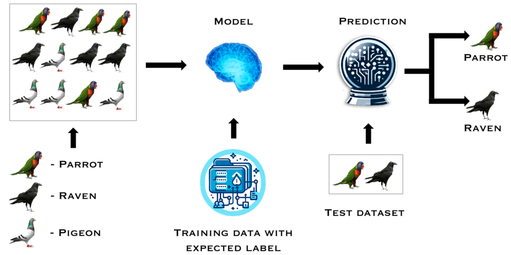
Figure 1
📌 Key Components of Supervised Learning
- Test Dataset: A separate dataset used to evaluate the model’s performance.
- Training Dataset: The portion of data used to train the model.
- Features: Attributes or independent variables used to train the model. Example: House size, number of bedrooms, and location in a house price prediction model.
- Label: The value the model aims to predict. Example: The price of the house.
📌 How Supervised Learning Works
Supervised learning follows a structured pipeline:
- Collecting Data: Gathering labeled datasets relevant to the problem.
- Preprocessing the Data: Cleaning the data, handling missing values, and normalizing features.
- Feature Selection: Identifying the most relevant features for prediction.
- Training the Model: Feeding labeled data into the model for learning.
- Evaluating the Model: Testing the model on new data to check accuracy.
- Making Predictions: Applying the trained model to unseen data.
Figure 2 illustrates a sample dataset that includes features and label.
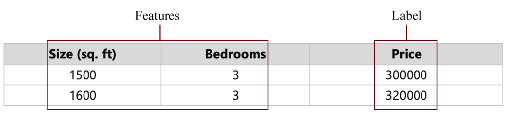
Figure 2
Key Supervised Learning Algorithms
Several supervised learning algorithms help with different types of problems:
- Linear Regression: Predicting continuous values.
- Decision Trees: Splitting data into logical decision-based groups.
- Neural Networks: Mimicking the human brain for complex data learning.
- Support Vector Machines (SVM): Classifying data points by finding the best separation boundary.
📌 Linear Regression
It is one of the most straightforward techniques in supervised learning. It is a mathematical model that shows the dependence among the factors we try to forecast in case there is an interrelation between them. Supported by those data, a linear equation can be formed between dependent and independent variables, demonstrating their relationship, as shown in Figure 3. It is how the linear equation can be written:
𝑦 = 𝛽0+𝛽1𝑥1+⋯+𝛽𝑛𝑥𝑛
- 𝑦 – The predicted value.
- 𝛽0 – The intercept.
- 𝛽i – The coefficient determining the influence of each feature xi.
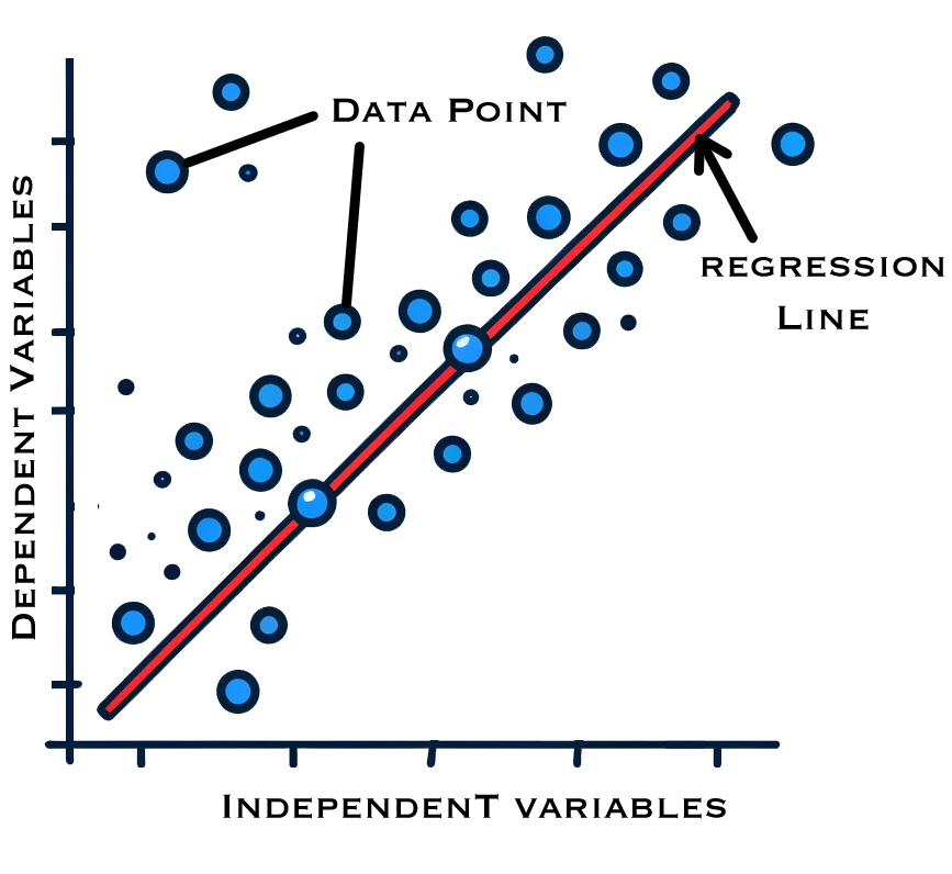
Figure 3
Real World Applications
- Real Estate: Predicting house prices based on size and location.
- Finance: Forecasting stock prices and sales revenue.
- Marketing: Estimating customer demand for products.
📌 Decision Trees
Decision trees are structured like a flowchart, where each node represents a decision based on a feature. These are non-parametric supervised learning methods for classification and regression tasks, as shown in Figure 4.
- Root Node: The main decision point.
- Branches: Different paths based on feature conditions.
- Leaves: Final decision or classification.
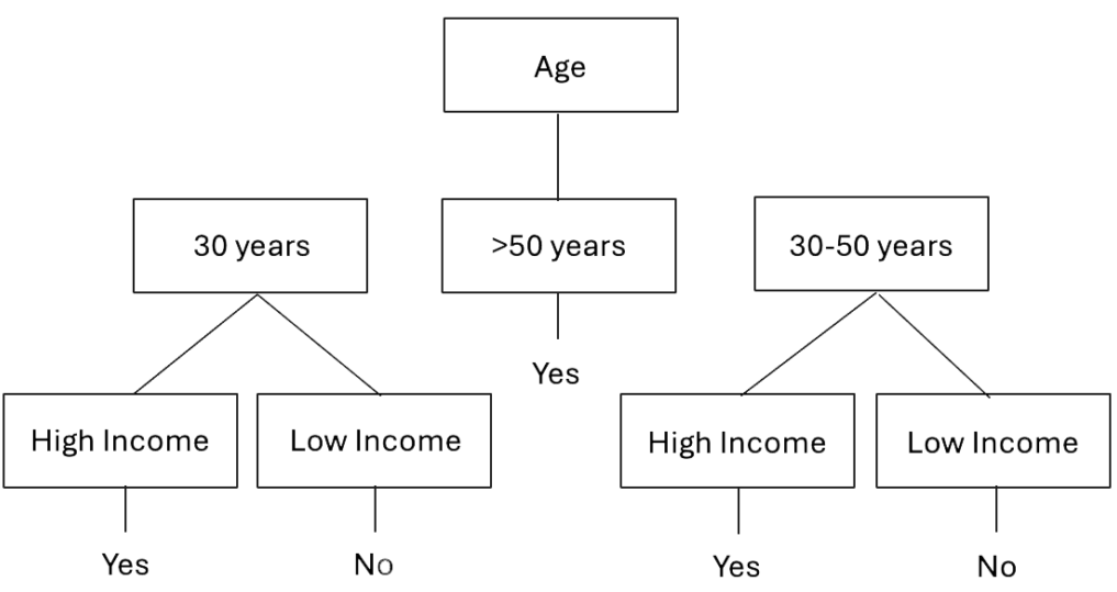
Figure 4
Real World Applications
- Healthcare: Diagnosing diseases based on symptoms.
- Finance: Credit risk assessment and fraud detection.
- Marketing: Customer segmentation and personalized ads.
📌 Neural Networks: Learning Like the Human Brain
Neural networks, particularly deep learning models, are designed to identify patterns in data like the human brain, as illustrated in Figure 5. They are generally defined as three layers.
- Input Layer: Receives the raw data.
- Hidden Layers: Transforms data through weighted connections.
- Output Layer: Produces the final prediction.
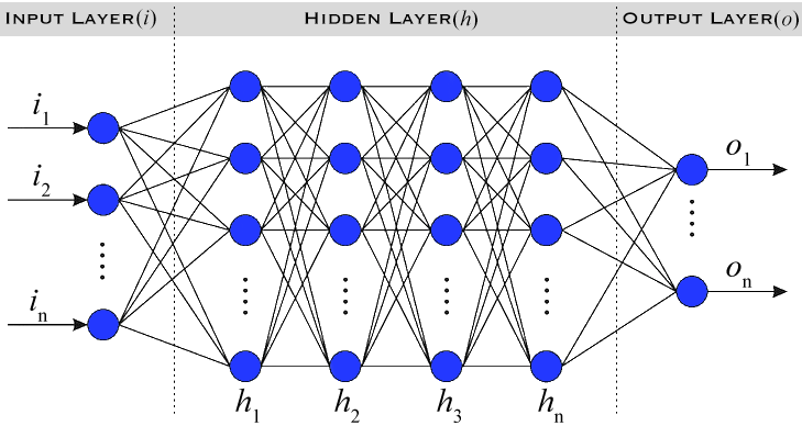
Figure 5
Real World Applications
- Healthcare: Disease diagnosis and medical image analysis.
- Finance: Fraud detection and stock market prediction.
- E-Commerce: Chatbots and product recommendations.
📌 Support Vector Machines (SVM)
SVM is a powerful classification algorithm that finds the optimal hyperplane separating different classes, as shown in Figure 6. There are two types of SVM.
- Linear SVM: Used when data is separable by a straight line.
- Non-Linear SVM: Uses kernel tricks to map data into a higher-dimensional space.
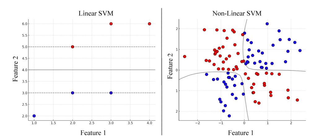
Figure 6
Real World Applications
- Marketing: Customer segmentation and sentiment analysis.
- E-Commerce: Spam detection in product reviews.
- Cybersecurity: Intrusion detection and malware classification.
- Natural Language Processing: Handwriting and speech recognition.
Advantages and Challenges of Supervised Learning
Advantages
- High Accuracy: Produces reliable predictions.
- Clearly Labeled Data: Well-defined input-output relationships.
- Effective in Many Applications: Used in finance, healthcare, and more.
Challenges
- Requires a Large Labeled Dataset: Labeling data is time-consuming.
- Risk of Overfitting: The model may memorize training data instead of generalizing.
- Computational Cost: Training complex models requires significant resources.
How to perform supervised learning?
- Collecting Data: All this information, including features and label data, has to be added.
- Preprocessing the data: Cleaning, handling data filled with missing values and variables, etc.
- Choosing Features: Decide which features are relevant to the prediction process and the most suitable ones.
- Training model: Use the training dataset, which consists of features with labels, to train the model.
- Evaluating the model: This procedure is most important because the testing data should be different from the training dataset to validate how precise a model can be.
- Prediction: The model inserted is applied to predict based on new data that follows the patterns of the process.
📌 Practical Example: Predicting House Prices
Step-by-step:
- Problem Definition: We aim to predict house price based on size and bedrooms. A sample dataset is shown in Table 1.
- Features: In this example, the features could include Size (sq. ft.) and Bedrooms
- Label: In this example, the label is Price.
| Size (sq. ft.) | Bedrooms | Price |
|---|---|---|
| 1500 | 3 | 300000 |
| 1600 | 3 | 320000 |
| 1700 | 3 | 340000 |
| 1800 | 4 | 360000 |
| 1900 | 4 | 380000 |
| 2000 | 4 | 400000 |
| 2100 | 5 | 420000 |
| 2200 | 5 | 440000 |
| 2300 | 5 | 460000 |
| 2400 | 5 | 480000 |
Table 1
We will implement this using linear regression in Python with the scikit-learn library, a popular tool for simple and effective modeling.
import numpy as np
import pandas as pd
from sklearn.model_selection import train_test_split
from sklearn.linear_model import LinearRegression
from sklearn.metrics import mean_squared_error, r2_score

# Sample dataset
data = {
    'Size': [1500, 1600, 1700, 1800, 1900, 2000, 2100, 2200, 2300, 2400],
    'Bedrooms': [3, 3, 3, 4, 4, 4, 5, 5, 5, 5],
    'Price': [300000, 320000, 340000, 360000, 380000, 400000, 420000, 440000, 460000, 480000]
}

# Creating DataFrame
df = pd.DataFrame(data)

# Features and target
X = df[['Size', 'Bedrooms']]
y = df['Price']

# Splitting data into training and testing sets
X_train, X_test, y_train, y_test = train_test_split(X, y, test_size=0.2, random_state=42)

# Initializing and training the model
model = LinearRegression()
model.fit(X_train, y_train)

# Making predictions
y_pred = model.predict(X_test)

# Evaluating the model
mse = mean_squared_error(y_test, y_pred)
r2 = r2_score(y_test, y_pred)

# Displaying the results
print(f"Mean Squared Error: {mse}")
print(f"R-squared: {r2}")

# Sample prediction
sample_data = np.array([[2100, 5]])
predicted_price = model.predict(sample_data)
print(f"Predicted price for house with 2100 sq.ft and 5 bedrooms: ${predicted_price[0]:.2f}")
Explanation:
- Making a Dataset: We will have a simple but practical data set with the bedroom count, house size, and house price as fields.
- Preprocessing the data: Pandas data frame (in Python code) is employed to carry out the data frame and indicate features (size, bedroom) along with the label (price).
- Model Training: We used the train_test_split process to separate the dataset into training and testing datasets. We then constituted training data for the linear regression model and trained it.
- Test Set: The model will be tested, based on the test dataset for prediction accuracy.
- Evaluating the model: Use two metrics (MSE and R²) to evaluate the model’s strength.
- Ask the question: What is the cost of a house with 2100 sq. ft and 5 bedrooms?