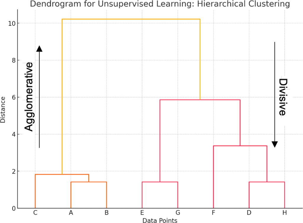
Hierarchical clustering is one of the clustering methods in unsupervised learning, which aims to create a tree of clusters. Unlike other clustering methods, hierarchical clustering does not have to decide the number of clusters in advance. Instead, it makes a graphical representation in the form of a tree structure that is well known as a dendrogram to demonstrate data and their clustering hierarchy, as shown in Figure 1. There are two main types of hierarchical clustering: agglomerative, also referred to as the bottom-up approach, and divisive, or the top-down approach.

Figure 1

Agglomerative (Bottom-Up)

Agglomerative hierarchical clustering is a procedure where each object is treated as a cluster of its own, and new clusters are formed by merging smaller clusters to move up the hierarchy level. This process is continued until all data points are contained in a single cluster. The output of this method is usually represented in the form of a dendrogram, which represents how clusters were merged in terms of distance.

Steps in agglomerative hierarchical clustering:

• Initialization: Begin with each data point forming its cluster.
• Compute distance matrix: The distance between two data points is computed using pairwise elements in the given data set. Common distance measures are the Euclidean distance, the Manhattan distance, and so on.
• Merge clusters: Find which of the previously calculated clusters is nearest to each other according to the selected distance measure and merge them.
• Update distance matrix: This step recalculates the distances between the new cluster and the other remaining clusters, modifying the distance matrix to form the new clusters.
• Repeat: Proceed with the next steps of merging the nearest clusters and modifying the distances until all the clusters are combined.
• Construct Dendrogram: The merging steps are recorded and employed to develop a dendrogram to illustrate the continuous pattern regarding clusters.

Linkage criteria:

• Single linkage (minimum): The feature measures the distance between the nearest points of the two clusters.
• Complete linkage (maximum): The maximum distance between two sites that belong to distinct clusters.
• Average linkage: The average separation between every point in the two clusters.
• Centroid linkage: The average difference between the centroids, which stand for the mean center of the two clusters.

Practical example:

Suppose we have a set of fruits, and we desire to classify those fruits on specific attributes like sweetness, crunchiness, and juiciness, among others. We then process each fruit as a single cluster and combine clusters as the analysis progresses.

import numpy as np
import matplotlib.pyplot as plt
from scipy.cluster.hierarchy import dendrogram, linkage

# Example dataset of fruits
# Encoding: [Sweetness, Crunchiness, Juiciness]
data = np.array([
    [8, 5, 2],  # Apple
    [7, 6, 1],  # Pear
    [6, 8, 1],  # Carrot
    [5, 2, 9],  # Watermelon
    [9, 3, 8],  # Mango
    [7, 2, 6],  # Banana
    [4, 7, 2],  # Cucumber
    [8, 4, 3],  # Pineapple
])

# Labels for the data points for clarity
labels = ["Apple", "Pear", "Carrot", "Watermelon", "Mango", "Banana", "Cucumber", "Pineapple"]

# Perform agglomerative hierarchical clustering
# Using 'ward' linkage method for this example to minimize the variance within clusters
Z = linkage(data, method='ward')

# Create a dendrogram
plt.figure(figsize=(10, 7))
dendrogram(Z, labels=labels)
plt.title("Dendrogram for Agglomerative Hierarchical Clustering of Fruits")
plt.xlabel("Fruits")
plt.ylabel("Distance")
plt.show()

Explanation:

• Dataset: The juice, crunch, and sweet categories are based on a fruit’s three basic attributes. Thus, each fruit will be depicted as an object belonging to a three-dimensional tuple characterized by specific properties.
• Agglomerative clustering: The given data set is used for performing agglomerative hierarchical analysis, and the Python linkage function (scipy.cluster.hierarchy) is applied. When forming a cluster for linkage, the ward technique assists in reducing the amount of variance in clusters; it is used when the features are purely numbers and can help develop an equal number of clusters.
• Dendrogram plotting: Hierarchical clustering is done, and this is depicted with the help of a dendrogram made with the dendrogram function. The fruits are shown on the X-axis, and the distance between the cluster mergers is depicted on the Y-axis. The splits involved in the dendrogram are as follows: Each of the splits demonstrates how the small groups can be related in terms of the formation of clusters.

Divisive (Top-Down)

It is a procedure in cluster analysis that is performed from a top-down approach. The technique of agglomerative clustering combines the objects to form larger clusters. Divisive clustering starts with each object as its own cluster and divides it into two or more clusters. It goes on until there is a single cluster per data point.

Steps in divisive hierarchical clustering:

• Initialization: To initialize, place all the data points in a single cluster.
• Splitting: Specify a cluster to split. This can be done using various rules based on the largest cluster or the cluster’s variance value.
• Determine split: Determine how the chosen cluster should be divided to achieve two smaller clusters. This can be achieved by k-means or by determining the point that maximizes the between-cluster variance.
• Update clusters: Further divide the identified cluster into two new clusters.
• Repeat: Repeat the process of choosing clusters, splitting them, and finding the best split until every data point is the cluster itself or until the pre-decided stopping criterion (like the number of clusters) is reached.

Practical example:

Now, let’s perform a primitive case of divisive hierarchical clustering based on the description of students being divided into groups by their favorite subjects and then further divided according to the specific interests within these groups.

# Example dataset of students
# Encoding: Humanities: 0, Science: 1
# Within Science: Physics: 2, Chemistry: 3, Biology: 4
# Within Humanities: Literature: 5, History: 6, Art: 7
data = np.array([
    [0, 5], [0, 6], [0, 7],  # Humanities: Literature, History, Art
    [1, 2], [1, 2], [1, 3], [1, 3], [1, 4], [1, 4], [1, 4]  # Science: Physics, Chemistry, Biology
])

# Labels for the data points for clarity
labels = ["Student 1", "Student 2", "Student 3", "Student 4", "Student 5", 
          "Student 6", "Student 7", "Student 8", "Student 9", "Student 10"]

# Function to perform divisive clustering and keep track of splits
def divisive_clustering(data, label_list, depth=0, max_depth=10):
    if len(data) <= 1 or depth >= max_depth:
        return
    
    # Perform KMeans clustering to split into 2 clusters
    kmeans = KMeans(n_clusters=2, random_state=0).fit(data)
    cluster_labels = kmeans.labels_
    
    # Split data and label lists
    left_data = data[cluster_labels == 0]
    right_data = data[cluster_labels == 1]
    left_labels = label_list[cluster_labels == 0]
    right_labels = label_list[cluster_labels == 1]
    
    # Record the split
    if len(left_labels) > 0 and len(right_labels) > 0:
        splits.append((left_labels.tolist(), right_labels.tolist()))
    
    # Recursively cluster the splits
    divisive_clustering(left_data, left_labels, depth + 1, max_depth)
    divisive_clustering(right_data, right_labels, depth + 1, max_depth)

# Initialize a list to keep track of splits
splits = []
divisive_clustering(data, np.array(labels))

# Function to create a custom dendrogram from the splits
def plot_custom_dendrogram(splits):
    fig, ax = plt.subplots(figsize=(10, 7))
    y_positions = {label: i for i, label in enumerate(sum(splits[0], []))}
    
    for i, (left, right) in enumerate(splits):
        if left and right:
            y_left = [y_positions[label] for label in left]
            y_right = [y_positions[label] for label in right]
        
            y_mid = (max(y_left) + min(y_right)) / 2
            for label in left + right:
                y_positions[label] = y_mid
        
            ax.plot([i, i], [min(y_left), max(y_left)], 'k-')
            ax.plot([i, i], [min(y_right), max(y_right)], 'k-')
            ax.plot([i, i + 1], [max(y_left), max(y_left)], 'k-')
            ax.plot([i, i + 1], [min(y_right), min(y_right)], 'k-')
    
    ax.set_yticks(range(len(labels)))
    ax.set_yticklabels(labels)
    ax.set_title("Custom Dendrogram for Divisive Hierarchical Clustering of Students")
    ax.set_xlabel("Splits")
    ax.set_ylabel("Students")
    plt.show()

# Plot the custom dendrogram
plot_custom_dendrogram(splits)

Explanation:

• Dataset: The students’ preferences are described in the dataset. The first number is the separate category that was requested (0 for humanities, 1 for science), and the second number states the interest within that category.
• Recursive divisive clustering function: The divisive_clustering function applies k-means with 𝑘=2, which splits data into two clusters. It updates cluster_labels with new cluster labels, which are recursively split until each student is in its cluster.
• Cluster label initialization: We create an array of cluster_labels, which will store the cluster labels for each student.
• Perform clustering: To perform the clustering, we are now calling the function called “divisive_clustering” on the dataset.
• Dendrogram plotting: We plot a dendrogram using the plot_custom_dendrogram function, which generates the dendrogram based on the linkage matrix. This helps us understand the pattern of clustering.