Introduction to Unsupervised Learning
Unsupervised learning is a type of machine learning where the model finds patterns and relationships in data without predefined labels. Unlike supervised learning, where models learn from labeled datasets, unsupervised learning explores the underlying structure of raw data without human intervention, as shown in Figure 1.
This makes unsupervised learning particularly useful for data analysis, pattern recognition, and anomaly detection. Businesses and researchers use these techniques to segment customers, detect fraud, and improve recommendations.
The primary goal of unsupervised learning is to analyze data and uncover hidden structures. By linking distinct data points and aggregating information, unsupervised learning provides insights that might not be immediately visible.
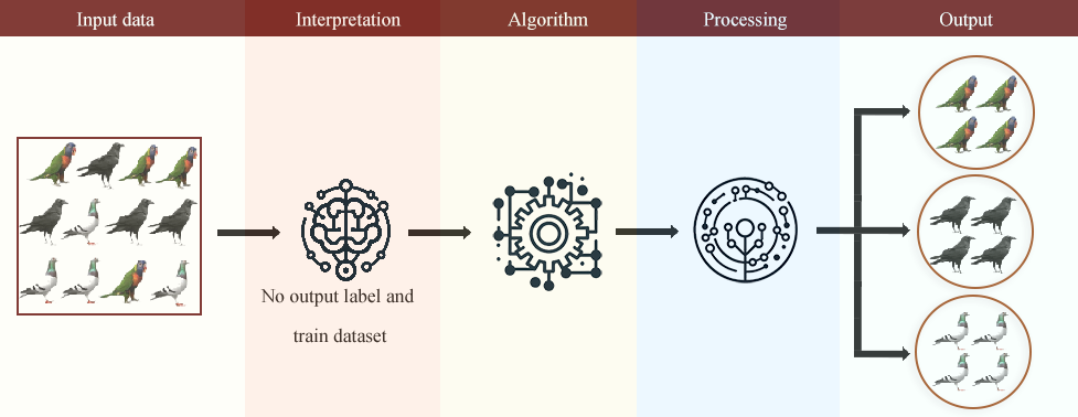
Figure 1
Key Techniques in Unsupervised Learning
There are three main approaches to unsupervised learning:
- Clustering: Grouping similar data points together.
- Dimensionality Reduction: Simplifying data while retaining its essential features.
- Association Rule Learning: Identifying relationships between different data points.
📌 Clustering: Finding Natural Groupings in Data
Clustering is the process of dividing a dataset into groups, where data points within the same group are more similar to each other than to those in other groups, as shown in Figure 2. This is particularly useful for:
- Customer segmentation: Grouping customers based on purchasing behavior.
- Medical research: Identifying different genetic disorders.
- Anomaly detection: Finding unusual patterns in financial transactions.
Popular Clustering Algorithms
- K-Means Clustering: Assigns data points to the closest cluster center.
- Hierarchical Clustering: Builds a hierarchy of clusters for better interpretability.
- Gaussian Mixture Models (GMM): Uses probability distributions to create flexible clusters.
- Density-Based Spatial Clustering of Applications with Noise (DBSCAN): Identifies dense areas of data while ignoring noise.
- Self-Organizing Maps (SOM): A neural network-based clustering method.
- Spectral Clustering: Uses graph theory to cluster complex data structures.
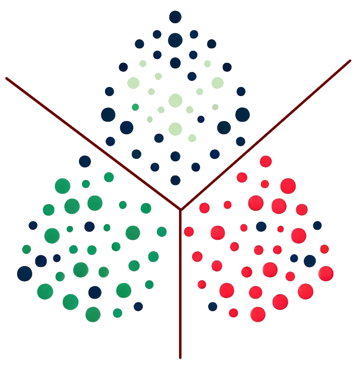
Figure 2
📌 Dimensionality Reduction: Simplifying Complex Data
Dimensionality reduction helps in reducing the number of input variables while preserving essential information, as shown in Figure 3. This is useful in:
- Image compression: Reducing the storage size of images while maintaining clarity.
- Feature selection: Identifying the most important factors in machine learning models.
- Big data visualization: Making complex datasets easier to understand.
Common Dimensionality Reduction Techniques
- Principal Component Analysis (PCA): Transforms high-dimensional data into fewer dimensions.
- t-Distributed Stochastic Neighbor Embedding (t-SNE): Visualizes complex datasets in 2D/3D.
- Autoencoders: Neural networks that encode and decode data for feature reduction.
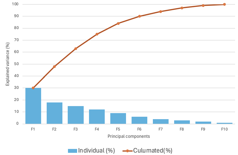
Figure 3
📌 Association rule learning
Association rule learning identifies patterns in data that show how different items are related. This is especially useful in:
- Market basket analysis: Identifying products frequently bought together in retail.
- Recommendation systems: Suggesting movies, books, or products based on past behavior.
- Medical research: Detecting relationships between symptoms and diseases.
Popular Association Rule Learning Techniques
- Apriori Algorithm: Finds frequent itemsets in transactional data.
- Eclat Algorithm: A faster alternative to Apriori for rule discovery.
- Market Basket Analysis: Commonly used in retail to suggest products frequently bought together.
Example: If among 100 transactions containing ‘bread’, we also have ‘butter’ in 75 of them, then the confidence of the rule {bread} ➞ {butter} is 75/100 * 100 = 75%.
Sample rule table
| Rule | Support | Confidence |
|---|---|---|
| If a customer buys bread, they are likely to buy butter. | 20% | 75% |
| If a customer buys a laptop, they are likely to buy a laptop bag. | 15% | 80% |
| If a customer views a smartphone, they are likely to view a smartphone case. | 10% | 60% |
| If a customer buys milk, they are likely to buy eggs. | 25% | 65% |
Practical example 1 (Step-by-step):
- Dimensionality Reduction: Rescale a high-dimensional dataset using PCA or autoencoders to ease its analysis and visualization.
- Clustering: The clustering (e.g., K-means) was performed on the reduced data to identify distinct groups.
- Association Rule Learning: Each cluster applies association rule mining to identify the relationships and rules describing the data.
import numpy as np
from sklearn.decomposition import PCA
from sklearn.cluster import KMeans
from mlxtend.preprocessing import TransactionEncoder
from mlxtend.frequent_patterns import apriori, association_rules
import pandas as pd
# Step 1: Dimensionality Reduction
np.random.seed(42)
X = np.random.rand(100, 10)
pca = PCA(n_components=2)
X_reduced = pca.fit_transform(X)
# Step 2: Clustering
kmeans = KMeans(n_clusters=3, random_state=42)
clusters = kmeans.fit_predict(X_reduced)
# Step 3: Association Rule Learning
# Generating sample transaction data based on clusters
transactions = []
for cluster in range(3):
    cluster_data = X[clusters == cluster]
    transactions.append((cluster_data > 0.5).astype(int).tolist())
transactions = [item for sublist in transactions for item in sublist]
te = TransactionEncoder()
te_ary = te.fit(transactions).transform(transactions)
df = pd.DataFrame(te_ary, columns=te.columns_)
frequent_itemsets = apriori(df, min_support=0.2, use_colnames=True)
rules = association_rules(frequent_itemsets, metric="confidence", min_threshold=0.6)
print(rules)
Explanation:
- Dimensionality Reduction: PCA is applied to keep only two dimensions representing the dataset we are dealing with.
- Clustering: Applying K-means clustering to get 3 clusters in the reduced data.
- Association Rule Learning: This data in each cluster is considered transactions to derive the frequent itemsets and association rules.
Practical example 2 (Step-by-step):
In the following example, I will use the Keras library to build an autoencoder and learn features with clusters. Autoencoders are among the most preferred for unsupervised learning since they can effectively learn a compressed data representation for clustering.
- Data Preparation: Import the dataset and prepare the training and test data. In this example, we will use the MNIST dataset.
- Build the Autoencoder: Create the encoder model to compress the input data. Based on the compressed form, design an algorithm for decoding the original data.
- Train the Autoencoder: Train the autoencoder to minimize the reconstruction error.
- Extract Features: Feature extraction process with the use of the encoder part of the autoencoder.
- Clustering: Perform an application of a clustering algorithm (e.g., K-Means).
- Evaluate the Clustering: Visualize the clusters to understand the clustering quality.
import numpy as np
import matplotlib.pyplot as plt
from keras.datasets import mnist
from keras.models import Model
from keras.layers import Input, Dense
from keras.optimizers import Adam
from sklearn.cluster import KMeans
from sklearn.manifold import TSNE
# Step 1: Load and preprocess the dataset
(x_train, _), (x_test, _) = mnist.load_data()
x_train = x_train.astype('float32') / 255.0
x_test = x_test.astype('float32') / 255.0
x_train = x_train.reshape((len(x_train), np.prod(x_train.shape[1:])))
x_test = x_test.reshape((len(x_test), np.prod(x_test.shape[1:])))
# Step 2: Build the autoencoder
input_dim = x_train.shape[1]
encoding_dim = 64  # Size of the encoded representation
input_img = Input(shape=(input_dim,))
encoded = Dense(encoding_dim, activation='relu')(input_img)
decoded = Dense(input_dim, activation='sigmoid')(encoded)
autoencoder = Model(input_img, decoded)
encoder = Model(input_img, encoded)
encoded_input = Input(shape=(encoding_dim,))
decoder_layer = autoencoder.layers[-1]
decoder = Model(encoded_input, decoder_layer(encoded_input))
autoencoder.compile(optimizer=Adam(), loss='binary_crossentropy')
# Step 3: Train the autoencoder
autoencoder.fit(x_train, x_train,
                epochs=50,
                batch_size=256,
                shuffle=True,
                validation_data=(x_test, x_test))
# Step 4: Extract features
encoded_imgs = encoder.predict(x_train)
# Step 5: Apply KMeans clustering
n_clusters = 10
kmeans = KMeans(n_clusters=n_clusters, random_state=42)
kmeans.fit(encoded_imgs)
y_kmeans = kmeans.predict(encoded_imgs)
# Step 6: Visualize the clusters using t-SNE
tsne = TSNE(n_components=2, random_state=42)
encoded_imgs_2d = tsne.fit_transform(encoded_imgs)
plt.figure(figsize=(8, 8))
for i in range(n_clusters):
    plt.scatter(encoded_imgs_2d[y_kmeans == i, 0], encoded_imgs_2d[y_kmeans == i, 1], label=f'Cluster {i}')
plt.legend()
plt.show()
Explanation:
- Data Preparation: Data preprocessing is done on MNIST (Modified National Institute of Standards and Technology), which is the most frequently used dataset in the deep learning community concerning the image of handwritten digits from 0 to 9. It is mostly used for training and learning neural networks with image processing, particularly for handwritten number recognition.
- Build the Autoencoder: This architecture usually comprises an encoder and a decoder network. The encoder compresses the input data to a lower dimension as compared to that of the input. The decoder takes in the encoded data and reconstructs the input data.
- Train the Autoencoder: Autoencoder training is usually done using the Adam optimizer to minimize reconstruction errors.
- Extract Features: The encoder transforms the input data into the encoded representation after training.
- Clustering: K-means clustering is performed on the encoded feature in order to obtain clusters of this data.
- Evaluate the Clustering: The 2D format is achieved by using t-SNE to encode the features. The clusters are plotted to see if the clustering results are proper.
This example shows how deep learning can be used in clustering by extracting a compressed feature of a dataset through an autoencoder and then applying a clustering algorithm to the learned features.